The Patterns of Chaos
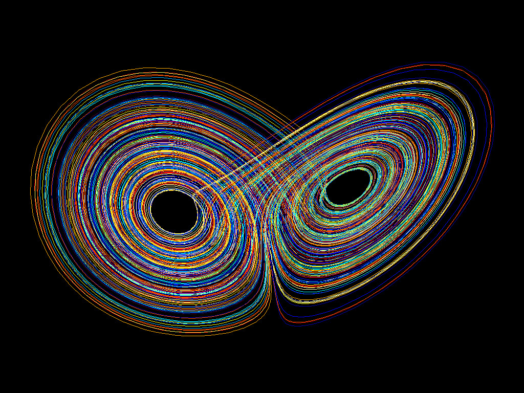
Table of Contents
An Experiment in Chaos Theory
On a cold winter day 60 years ago, Edward Lorenz was running an experiment on his computer simulation of weather patterns. After entering some numbers and going out to get coffee for ten minutes, he noticed something weird in the results when he returned. He noticed what would be infamously known as the chaos theory — a discovery that would change science forever!
His computer model was a combination of 12 variables, each representing a different aspect of the weather, such as temperature and wind speed. Lorenz was repeating a simulation that he had run earlier. However, when Edward Lorenz rounded off one variable from .506127 to .506 in his program, it altered the entire pattern of simulated weather projections over the next two months. Under normal parameters and given the same starting point, the weather would unfold exactly the same way each time. A slightly different starting point should unfold in a slightly different way. An error of a few degrees would surely be insignificant to change anything at a large scale.
During that time, the assumption at the heart of science was that given an understanding of the laws of physics and a system’s initial conditions, one could calculate the approximate behavior of a closed system. The idea of science was that the falling of a leaf on some planet in another galaxy could not affect the movement of a billiard ball on earth. The belief was that small changes don’t blow up into larger effects in that smaller causes yield smaller effects.
The French mathematician Pierre-Simon Laplace remarked in his 1814 volume A Philosophical Essay on Probabilities that if we knew everything about the universe in its present state, then “nothing would be uncertain and the future, as the past, would be present to [our] eyes.”
Yet, in Edward Lorenz’s particular system of differential equations, small errors cascaded into unfathomable changes over time. The questions stared at him, and he had no answers. What if apparent randomness could come from simple models? What if the same simple models in one system gave birth to complexity in another? What if randomness or chaos was the norm rather than a byproduct of measurement inefficiencies? What if chaos wasn’t the inability of observation but the substratum of the natural law itself?

Fig- Two simulated weather patterns running over a period of two months.
The unexpected result led Lorenz to realize that small changes could have large effects— a powerful insight into how nature worked. The idea became known to be the Butterfly Effect. Chaos theory, or the butterfly effect, is the idea that small changes have the potential to cause major changes across chaotic systems. Edward Lorenz coined the term after he hypothesized that a distant butterfly’s flapping wings could set off a complex series of events, leading to a tornado somewhere else.
Lorenz realized that sensitivity to initial conditions is what causes nonperiodic behavior. The effect later acquired a technical name: the sensitive dependence on initial conditions. Yet, a look at folklore reveals that the poets of old had already known and answered what chaos theory is:
“For want of a nail, the shoe was lost;
For want of a shoe, the horse was lost;
For want of a horse, the rider was lost;
For want of a rider, the battle was lost;
For want of a battle, the kingdom was lost!”
Chaos Theory Explained: The Science of Chaos
As James Gleick says in his book Chaos, “WHERE CHAOS BEGINS,” classical science stops. For as long as the world has had physicists inquiring into the laws of nature, it has suffered a special ignorance about disorder in the atmosphere, in the turbulent sea, in the fluctuations of wildlife populations, in the oscillations of the heart and the brain. The irregular side of nature, the discontinuous and erratic side.”
The science of chaos has birthed its own language, comprising words like fractals, turbulence, periodicity, bifurcations, strange attractors, butterfly effect, and sensitive dependence. Such words represent a world where the rules are different — things branch into strange structures, following a pattern and periodicity that can be known but impossible to precisely quantify and predict. If referenced through the prism of a space-time continuum, it is as if everything of this chaotic world folds back on itself to be both the future and past simultaneously — drawing its periodicity from itself. A chaos that is not the rejection of order but its natural expression.
The science of chaos seems to answer some of the most fundamental questions humanity struggles to answer: How does life begin? What is turbulence? Above all, in a universe governed by entropy, which creates greater disorder, how does order arise? A science that addresses the age-old question: how does the microcosm weave itself into the macrocosm? When studied in isolation, one atom or neuron behaves in one way, but billions of atoms and neurons behave completely differently. A science that unravels the link between aperiodicity and unpredictability.
What Is Chaos Theory?
At the heart of chaos is the study of nonlinearity, which entails that playing the game can change the rules. Nonlinearity makes understanding non-linear things difficult because of existing twisted changeability between different variables, creating rich and complex behaviors. For instance, one cannot assign constant importance to friction because its importance depends on speed. Speed, in turn, depends on friction. Therefore quantifying nonlinearity is like solving a Rubik’s cube whose colors change every time you make a move.
Let’s consider some of the most common everyday examples:
Predicting Weather
Given major technological innovations over the past two centuries, weather forecasting in the short run has dramatically improved. But predicting weather conditions, in the long run, can be tricky. Most modern weather models, even the AI-powered ones, work with a grid of geographically monitored points spread across 10-200 km. To determine the weather, meteorologists use a series of differential equations to analyze raw data, which includes dew intensity, temperature, wind, and pressure, among other variables.
Some starting data, like moisture, has to be guessed since ground stations and satellites cannot observe everything. Mostly, the guesswork is reliable. But suppose we could upgrade the equipment to pinpoint accuracy and cover the entirety of earth with sensors spaced just a few feet apart in three-dimensional space. Suppose every sensor gives perfectly accurate readings that meteorologists are looking to observe. Suppose an AI-powered quantum computer takes all those readings and calculates the emergence of weather patterns at intervals of a few minutes. What would happen then? Would we be able to predict the weather with absolute precision?
We will observe that we can still not predict weather patterns for a specific place in the long run. The spaces between the sensors will hide micro fluctuations — stretching into the quantum realm — that the computer will not know about. These will be just tiny deviations from the average. And within minutes, those fluctuations will already have created small errors just a few feet away. Soon the multiplier effect would ensue, and the errors would add up, even at a distance of 10 feet. Hence, rendering it impossible to predict the weather with absolute accuracy.
A Hot Cup of Coffee and Chaos
Hot liquids are one of the many hydrodynamical processes governed by the laws of chaos. Take the example of a simple cup of coffee. How can we calculate how exactly and how quickly a cup of coffee will cool down? If the coffee is warm, its heat will dissipate without any hydrodynamic motion, hence not giving rise to turbulence. But what happens if the temperature rises to the point that the coffee starts boiling?
If you look closely at a hot cup of coffee, you will immediately notice on the surface of your drink dusty swirling white areas outlined by a dark line. These whirling patterns are called convection cells. These patterns mark areas where hot coffee rises to the surface, and slightly cooled coffee is pulled toward the bottom by gravitational force. Convection is a common process that occurs when warmer air or liquid lies under a cooler layer. This happens in the coffee cup: the coffee on top is cooled by evaporation, and as it cools down, it also becomes heavier and gets pulled down by gravity. Simultaneously, the warmer portion of the coffee at the bottom rises to the top to replace it.
When the warmer coffee rises to the top, a small portion of its water evaporates and then condenses as it interacts with the cooler air above the surface. These droplets are just the right size and weight to stay on the surface. So, little clouds look like a coating on top of the coffee. They look white because the water reflects light. The black lines are where the cooler coffee is sinking toward the bottom.
The swirls can be complicated. But eventually, we know what becomes of the system. As the heat dissipates further and friction slows down the moving fluid, the internal motion within the cup of coffee must stop. Remarking on the phenomena, Edward Lorenz once said, “We might have trouble forecasting the temperature of the coffee one minute in advance, but we should have little difficulty forecasting it an hour ahead.”
Under the textbook convection model, the temperature difference between the hot bottom and the cool top controls the system’s flow. In simpler words, heat moves towards the top without disturbing the tendency of the liquid to remain at rest.
However, when the heat is turned up, it is observed that as the fluid becomes hotter, it expands in size, and its density decreases, making it light enough to overcome friction and rise toward the surface. But if the heat is increased further, the behavior of the liquid grows more complex. The rolls begin to wobble paving the way for turbulence — as depicted in the figure above.
Thus a seemingly stable system, when exposed to small changes like heating it up a mere 0.001 degree, can transition from orderly convection into turbulent chaos within seconds — even though such systems are deterministic to the point that their end result is predictable. However, in the short run, the deterministic tendency of the system must concede to chaos, making it impossible to predict something as simple as the temperature of a cup of coffee. Such a system follows deterministic chaos, whose behavior can, in principle, be predicted. But unpredictability emerges ‘over time’ or when we zoom ‘in time’.
Patterns of Chaos
Patterns of chaos in nature are all around us. These patterns include but are not limited to fractals and turbulence in fluids, shapes such as spirals or two-dimensional Mandelbrot sets, or something as ordinary as the nested layers within an onion.
Chaos in nature is a fascinating study. Every bit of it, from the smallest snowflake to an entire galaxy, every sound and sight tells its own story that we can’t help but be captivated by because there are so many layers to explore! From how music echoes within buildings with different materials making up their structure, such as brick or glass, all the way down through smaller structures like cells where DNA stores information for future generations – chaos has patterns everywhere.
Nature is a tapestry woven with patterns of order and chaos. Let’s explore some of these patterns.
Lorenz System: Butterfly Effect and Strange Attractors In Chaos Theory
After Lorenz observed the sensitive dependence of weather patterns on initial conditions, his interest grew in the mathematics behind the chaos, leading him to discover the infamous Lorenz Equation. In March 1963, Lorenz wrote that he wanted to introduce ordinary differential equations that solved for deterministic non-periodic flow and finite-amplitude convection (deterministic chaos).
Lorenz found that when applying the Fourier Series to one of Rayleigh’s convection equations that all except three variables tended to zero. These three variables exhibited irregular, apparently non-periodic functions. He used these variables to construct a simple model based on the 2D representation of the earth’s atmosphere.
He took a set of differential equations for convection and stripped it to the bone. And even though Lorenz’s System did not fully model convection, he could abstract one feature of real-world convection: the circular motion of hot fluid rising up and around.
The Lorenz equations are given by:
dx/dt = X’ = σ(y − x)
dy/dt = Y’ = ρx − y − xz
dz/dt = Z’ = xy − βz
The Lorenz equations contain three parameters: σ, ρ, β. In what follows, we will always assume that these parameters are positive. In all the numerical calculations below, we take σ = 10.0 and β = 8/3. The variable component is ρ. Here x, y, z do not refer to coordinates in space. X represents the convective overturning on the plane, while y and z are the horizontal and vertical temperature variations, respectively.
The parameters of this model are σ, which represents the ratio between the fluid viscosity to its thermal conductivity, ρ, which represents the difference in temperature between the top and bottom of the atmosphere plane, and β, which is the ratio of the width to the height of the plane.
Lorenz’s computer printed out the changing values of the three variables: 0–10–0; 4–12–0; 9–20–0; 16–36–2; 30–66–7; 54–115–24; 93–192–74. The three numbers rose and then fell as imaginary time intervals passed. Lorenz used each set of three numbers as coordinates to make a picture from the data. Thus the sequence of points created a map that showed how chaotic systems could change over time when one variable undergoes time-bound change.
The traditional expectation from the system was that it would either settle down into a steady state, where the variables for speed and temperature would no longer change, or the path might form a loop and settle into a pattern of behavior that would repeat itself periodically. Lorenz system did neither.

Fig- Lorenz System
The map formed a sense of infinite complexity that embodied chaos and order. It always stayed within certain bounds, but at the same time, it never repeated itself. The generated chaotic system moved predictably toward its attractor in phase space, but strange attractors appeared instead of points or simple loops. Strange attractors represent a chaotic system in a specific phase space, but attractors are also found in many nonchaotic dynamical systems.
The shape looked like a double spiral in three dimensions that looked like a butterfly. And thus came to be known as the butterfly effect.
Sample implementation of the differential equations for Lorenz Attractor (butterfly effect) in Java:
int i = 0;
double x0, y0, z0, x1, y1, z1;
double h = 0.01, a = 10.0, b = 28.0, c = 8.0 / 3.0;
x0 = 0.1;
y0 = 0;
z0 = 0;
for (i = 0; i < N; i++) {
x1 = x0 + h * a * (y0 – x0);
y1 = y0 + h * (x0 * (b – z0) – y0);
z1 = z0 + h * (x0 * y0 – c * z0);
x0 = x1;
y0 = y1;
z0 = z1;
// Printing the coordinates
if (i > 100)
System.out.println(i + ” ” + x0 + ” ” + y0 + ” ” + z0);
}
The Lorenz differential equations system established that order was hidden in the chaos. That chaos in itself couldn’t be reduced to randomness. The heart of chaos could finally be expressed through mathematical poetry. The math behind chaos established that the universe was governed by complex systems that simultaneously gave rise to turbulence and coherence — be it in the Great Red Spot of Jupiter or the population of species. The butterfly effect was the embodiment of chaos.
Feigenbaum Constant and the Chaos Theory
The mathematical representation of chaos established the importance of nonlinearity, a characteristic that governs most natural systems, including the gain in population. For instance, if a group of 1000 Elephants has a net gain of 10 members a year, that increase in population size can be represented as a straight line on a graph. However, a group of mice that doubles its population annually will have a nonlinear growth pattern — the graph can be represented as an upward curve. After a decade, the difference between the two mice groups (one with 22 mice and the other with 20 mice) will balloon to more than 2,000 due to the underlying nonlinearity of growth. Thus a non-linear growth pattern often causes animal population sizes to rise and fall chaotically.
One of the best ways to understand chaos theory is to look at animal populations. Let us assume that the equation xnext = rx(1-x) represents the growth of a population. Here, xnext represents the population for the next year, while x is the population for the existing year; r represents the growth rate, and (1-x) represents the factors keeping the growth within bounds. As x increases, (1-x) falls. Here, the population is expressed as a fraction between zero and one, where zero represents extinction, and one is the maximum possible population the species can attain. If the population falls below a certain level in one year, chances are it may increase next year. But if the population rises too much, competition within species for resources will tend to bring it within bounds.
The population will reach equilibrium after many initial fluctuations. The population gradually goes extinct when r attains small values. For bigger values of r, the population may converge to a single value. For even greater values, it may fluctuate between two values, and then four, and so on. But everything becomes unpredictable for greater values. The line representing the population function, though initially single, breaks into two, four…… and then goes chaotic. The population-versus-r graph for the situation produces an intriguing result.
When r is between 0 and 1, the population ultimately goes extinct. Between r = 1 to = 3, the population converges to a single value. At about r = 3.2, the graph bifurcates (breaks into two) since, at this value of r, the population does not converge to a single value but fluctuates between two values. For greater values of r, the bifurcation speeds up; and after a quick succession of period doublings soon, the graph becomes chaotic. This means that, for those corresponding values of r, the population fluctuates unpredictably between random values and never exhibits a periodic behavior. However, on closer inspection, it is evident that the graph becomes predictable at certain points between the chaotic portion. These can be called “windows of order amidst the chaos.” After the initial chaotic behavior, the chaos suddenly vanishes, leaving a stable period of three in its wake. This then continues to double – 6, 12, 24 and goes chaotic again… The chaotic behavior in the graph is a fractal. It shows how nonlinearities that are inherent in simple models for the regulation of plant and animal populations can lead to chaotic behavior.
Beyond a certain point, periodicity gives way to chaos, fluctuations that never settle down at all. Whole regions of the graph are completely blacked in. If you were following an animal population governed by this simplest nonlinear system of equations, you would come across complexity hidden as randomness. Yet, complexity doesn’t mean randomness. For every wild, uncontrollable change in animal population numbers, we observe there is a chain of events that returns year after year. Even though the parameter is rising, the nonlinearity drives the system harder and harder; a window will suddenly appear with a regular period: an odd period, like 3 or 7. The pattern of changing population repeats itself on a three-year or seven-year cycle. Then the period-doubling bifurcations begin all over at a faster rate, rapidly passing through cycles of 3, 6, 12…or 7, 14, 28…, and then breaking off once again to renewed chaos.

Fig- Population Bifurcation diagram.
On zooming in, it is evident that the chaotic part in the above graph repeats the same pattern endlessly. A fractal is a never-ending pattern. Fractals are infinitely complex patterns that are self-similar across different scales. They are created by repeating a simple process over and over in an ongoing feedback loop. In essence, a Fractal is a pattern that repeats forever, and every part of the Fractal, regardless of how zoomed in or zoomed out you are, looks very similar to the whole image. Driven by recursion, fractals are images of dynamic, chaotic systems – the pictures of Chaos. And as James Gleick puts it, “a way to look at infinity.”
After investigations, mathematician Mitchell Feigenbaum found that when he divided the width of each bifurcation section by that of the next one, their ratio converged to a constant value known as the Feigenbaum constant, 4.6692016090. For all bifurcation diagrams, no matter what function he used, the number remained the same. Scaling was the key. Feigenbaum believed that scaling (across different ranges) was the key to understanding perplexing phenomena like turbulence. Feigenbaum proposed the scenario called period doubling to describe the transition between regular dynamics and chaos. His proposal was based on the logistic map introduced by the biologist Robert M. May in 1976, who had found bifurcations while studying patterns boom-and–bustiness in animal populations.
Over time, it was also proven that the rules of complexity are universal and applied to all dynamical systems, regardless of their constituents. The behavior could be observed with a system as simple as dripping water from a faucet. Initially, water will fall drop-by-drop. Then, on speeding up the flow of the water, it will drip in pairs and so on, and then it follows a chaotic behaviour. This type of behavior applies to uncountable chaotic systems – from dripping water to amazingly complex Mandelbrot sets. Chaos is ubiquitous.
Mandelbrot Sets and Chaos Theory
Benoit Mandelbrot was a Polish-born French-American mathematician and polymath with broad interests in the practical sciences. He was largely responsible for the present interest in fractal geometry. He showed how fractals could occur in many different places in both mathematics and elsewhere in nature. Fractals have been employed to describe diverse behavior in economics, finance, the stock market, astronomy, and computer science. His contributions in fractal geometry have earned him the title ‘Father of Fractals.’
In 1961, Benoit Mandelbrot worked as a research scientist at the Thomas J. Watson Research Center in Yorktown Heights, NY. A bright young academic who had yet to find his professional niche, Mandelbrot was exactly the kind of intellectual maverick IBM had become known for recruiting. The task was simple enough: IBM was involved in transmitting computer data over phone lines, but a kind of white noise kept disturbing the flow of information—breaking the signal—and IBM looked to Mandelbrot to provide a new perspective on the problem.
Since he was a boy, Mandelbrot had always thought visually, so instead of using the established analytical techniques, he instinctually looked at the white noise in terms of the shapes it generated—an early form of IBM’s now-renowned data visualization practices. A graph of the turbulence quickly revealed a peculiar characteristic. Regardless of the scale of the graph, whether it represented data over the course of one day, one hour, or one second, the disturbance pattern was surprisingly similar. There was a larger structure at work. Periods of errorless communication were followed by periods of errors. Mandelbrot discovered a consistent geometric relationship between the bursts of errors and spaces of clean transmission. The transmission errors were like a Cantor set arranged in time. He classified the variation in terms of two kinds of effects: the Noah Effect and the Joseph Effect.

Fig- A Cantor Set
The Noah Effect means discontinuity: when a quantity changes, it can change almost arbitrarily fast. Economists traditionally imagined that prices change smoothly—rapidly or slowly, as the case may be, but smoothly in the sense that they pass through all the intervening levels on their way from one point to another. That motion image was borrowed from physics, like much of the mathematics applied to economics. But it was wrong. Prices can change in instantaneous jumps, as swiftly as a piece of news can flash across a teletype wire and a thousand brokers can change their minds. A stock market strategy was doomed to fail, Mandelbrot argued if it assumed that stock would have to sell for $50 at some point on its way down from $60 to $10.
The Joseph Effect means persistence. There came seven years of great plenty throughout the land of Egypt. And there shall arise after them seven years of famine. If the Biblical legend meant to imply periodicity, it was oversimplified, of course. But floods and droughts do persist. Despite underlying randomness, the longer a place has suffered drought, the likelier it is to suffer more. Furthermore, mathematical analysis of the Nile’s height showed persistence applied over centuries and decades. The Noah and Joseph Effects push in different directions, but they add up to this: natural trends are real, but they can vanish as quickly as they come.
Mandelbrot later turned his attention to measuring coastlines. How long was the coast of Britain? The answer, according to Mandelbrot, depended on the ruler one used. According to him, the coastline was infinitely long. A picture was forming in his head. But it was hazy. There was a pattern connecting the microcosm and the macrocosm. The roughness of the rocky shore looked the same when zoomed in or out from above. Mandelbrot was getting nearer to the realization that nature tends to repeat its patterns across different dimensions of measurement.
In 1945 Mandelbrot’s uncle introduced him to Julia’s important 1918 paper claiming that it was a masterpiece and a potential source of interesting problems, but Mandelbrot did not like it. Indeed he reacted rather badly against suggestions posed by his uncle since he felt that his whole attitude to mathematics was so different from that of his uncle. Instead, Mandelbrot chose his own very different course, which, however, brought him back to Julia’s paper while we was working for IBM.
Building on previous work by Gaston Julia and Pierre Fatou, Mandelbrot used a computer to plot images of the Julia sets. Investigating the topology of these Julia sets, patterns in cotton prices, frequency of electronic transmission noise, and repetition of river floods, Mandelbrot came to a realization that the irregular patterns in natural systems had a quality of self-similarity. There was symmetry across the scale — patterns inside patterns.
Mandelbrot built upon the work of Gaston Julia. Julia set fractals are normally generated by initializing a complex number z = x + yi where i2 = -1 and x and y are image pixel coordinates in the range of about -2 to 2. Then, z is repeatedly updated using: z = z2 + c, where c is another complex number that gives a specific Julia set. After numerous iterations, if the magnitude of z is less than 2, we say that pixel is in the Julia set and color it accordingly. Performing this calculation for a whole grid of pixels gives a fractal image.
Mandelbrot set the value of c to be x + yi, where x and y are the image coordinates (as was also used for the initial z value). This gave birth to the Mandelbrot set. The Mandelbrot set can be considered a map of all Julia sets because it uses a different c at each location as if transforming from one Julia set to another across space. The result was an awkwardly shaped bug-like formation, and it was perplexing, to say the least. Moreover, every smaller version held more complex detail than the previous version.
These structures were not exactly alike, but the general shape was strikingly similar; only the details differed. The specificity of these details, it turned out, was limited only to the power of the machine computing the equation, and similar shapes could continue on forever—revealing more and more detail, on an infinite scale. This was a definite geometry, there were rules and parameters to this roughness, but it was a form of geometry previously unidentified by the scientific community.

Fig- Mandelbrot Set
Mandelbrot set was introduced by Mandelbrot in 1979. In 1982, Mandelbrot expanded and updated his ideas in The Fractal Geometry of Nature. In this book, Mandelbrot highlighted the many occurrences of fractal objects in nature. The most basic example he gave was a tree. Each split in a tree—from trunk to limb to branch and so forth—was remarkably similar, he noted, yet with subtle differences that provided increasing detail, complexity, and insight into the inner workings of the tree as a whole. True to his academic roots, Mandelbrot went beyond identifying these natural instances and presented the sound mathematical theories and systems upon which his newly coined “fractal geometry” was based.
Chaos Theory Examples
Fractal patterns are everywhere: in mathematics, industry, the stock market, climate science, galaxies, trees, and even in the films we watch and the games we play. Multifractal patterns have been spotted in the quantum realm — at the atomic-scale resolution of a scanning tunneling microscope, the sudden transition at which material changes from a metal to an insulator, the waves associated with individual electrons gain a distinct multifractal pattern. Let’s look at some of the most astonishing patterns of chaos we’ve found in nature:
Jupiter’s Red Spot
Jupiter’s Red Spot is a thing of beauty in the study of chaos. The Great Red Spot is a storm in Jupiter’s southern hemisphere with crimson-colored clouds that spin counterclockwise at wind speeds that exceed those in any storm on Earth. Earthly hurricanes are powered by the heat released when moisture condenses to rain. The Red Spot is not powered by any such process. Hurricanes rotate in a cyclonic direction, counterclockwise above the Equator and clockwise below, like all earthly storms.
In contrast, the Red Spot’s rotation is anticyclonic. And most important, hurricanes die out within days. The Great Red Spot has been observed since 5 September 1831. The spot is a self-organizing system, regulated by the same turbulence that makes it chaotic. The paradoxical combination of stability amidst chaos creates this powerful storm with no end in sight.
The Human Body
Blood vessels, from the aorta to capillaries, form another kind of continuum; they branch and divide and branch again until they become so narrow that blood cells are forced to slide through a single file. The nature of their branching is fractal.
The lungs are an excellent example of a natural fractal organ. The volume of a pair of human lungs is only about 4-6 liters, but the surface area of the same pair of lungs is between 50-100 square meters. The lung surface area to volume ratio is very high and useful. This is possible only because the structure of the lungs is fractal. There are 11 orders of branching, from the trachea to the alveoli at the tips of the branches. Fractal branching geometry provides an incredibly useful way to make a very large surface area extremely compact.
Every cell in the body must be close to a blood vessel, say within about a hundred microns to be able to receive oxygen and nutrients. The fractal branching system of blood vessels down to the width of a capillary, which is about eight microns in diameter makes it possible. The length of blood vessels in the human body could be about 150,000 km of blood vessels as there are about 250 capillaries /mm3 of body tissue and the average length of a capillary is about six hundred microns.
Similarly, the brain’s neurons also possess a fractal pattern. The human brain comprises approximately 100 billion neurons with about 100 trillion synapses or connections among these neurons, and on average, each neuron may have to communicate with about a thousand cells at a time. The axons reach out to make synaptic connections with the dendrites of other neurons. It is the fractal branching pattern of the neuron’s axons and dendrites that allows them to communicate with so many other cells.
In fact, the fractal dimension of cancerous material is higher than that of healthy cells. Alan Penn, who is an Adjunct Professor of Mathematics and Engineering at George Washington University, describes his work in this area, “MRI Breast Imaging may improve diagnosis for the 4,000,000 women at risk for whom mammography isn’t effective. Clinical application of MRI has been hampered by difficulty in determining which masses are benign and which are malignant. Research has focused on developing robust fractal dimension estimates which will improve discrimination between benign and malignant breast masses.
The body structures of all of nature’s animals are fractal, and so too is their behaviour and even their timing. Our heartbeats seem regular and rhythmical, but when the timing structure is examined in fine detail, it is revealed to be slightly fractal. And this is very important. Our heartbeats are not regular. There is an important tiny variation. This fine variation reduces the wear and tear on the heart drastically. Just like the branches of a self-similar tree, the beats of the healthy human heart are statistically self-similar. Additionally, heart disease can be detected by extreme and arrhythmic fractal behavior.
Fractals in Nature
Fractal patterns are everywhere in nature. Examples are everywhere in the forest. Trees are natural fractals, patterns that repeat smaller and smaller copies of themselves to create the biodiversity of a forest. Each tree branch, from the trunk to the tips, is a copy of the one that came before it. This is a basic principle that we repeatedly see in the fractal structure of organic life forms throughout the natural systems in nature.
Flowers, Ferns, Leaves, River channels, Lightning, Snowflakes are some examples of fractals in nature. Romanesco Broccoli, a variant of cauliflower, is the ultimate fractal vegetable. Its pattern is a natural representation of the Fibonacci or golden spiral, a logarithmic spiral where every quarter turn is farther from the origin by a phi factor, the golden ratio.
The Fibonacci sequence, a common and beautiful numeric pattern in nature creates the Golden Ratio. Ferns are a common example of a self-similar set, meaning their pattern can be mathematically generated and reproduced at any magnification or reduction. The mathematical formula that describes ferns, named after Michael Barnsley, was one of the first to show that chaos is inherently unpredictable yet generally follows deterministic rules based on nonlinear iterative equations. In other words, random numbers generated over and over using Barnsley’s Fern formula ultimately produce a unique fern–shaped object. Many plants follow simple recursive formulas in generating their branching shapes and leaf patterns.
River deltas also tend to be fractal in nature. Even in the sky, analysis of satellite pictures has shown an invariant fractal dimension in clouds observed from hundreds of miles away. Lightning does not travel in straight lines but follows a chaotic behavior. Lightning can be very large, spanning several miles, but it is formed in microseconds. Thunder is a fractal sound. It is caused by the superheating of air. Because the pathway of the lightning bolt is a jagged fractal in 3D space, the time it takes to reach our ears varies, and hence the sound we hear is a fractal pattern.
Galaxies are the largest examples of spiral fractals known. A single spiral galaxy may contain a trillion stars. The spiral arms do not contain a greater number of stars, but they are still brighter because they contain many short-lived, extremely bright stars formed by a rotating spiral wave of star formation. The waves of star formation are made visible because they contain many young and very bright stars that only live a short time, perhaps 10 million years, as compared to the more common stars, such as our sun which live for several billion years.


Quantum Chaos
Quantum Chaos describes and tries to understand the nature of the wave-like motions of the electrons in atoms and molecules (quantum mechanics), as well as electromagnetic waves and acoustics, etc.. To a limited extent, these waves are like the chaotic trajectories of particles in classical mechanics, including the light rays in optical instruments and the sound waves in complicated containers. The study of quantum chaos encompasses applying dynamical systems theory in the quantum regime.
How does the macroscopic world we experience in everyday life emerge from the microscopic world invisible to the naked eye? This question, as old as science itself, became particularly relevant over the past 100 years in understanding how classical mechanics, governing the macroscopic world, derives from quantum mechanics, governing the underlying microscopic world. Although tremendous progress has been made, still many puzzling questions remain. The emergence of Chaos may well be the shared connection between the quantum world and the real world.
The central objective in the study of quantum chaos is to characterize universal properties of quantum systems that reflect the regular or chaotic features of the underlying classical dynamics. Researchers have observed that the latter universal property of classical chaos is intimately related to the universal spectral fluctuations characteristic of quantum chaos.
Quantum chaos began as an attempt to find chaos in quantum mechanical systems in extreme sensitivity to changes in initial conditions. That attempt failed since it was eventually realized that such sensitivity does not exist. However, along the way, it was found that chaos (or the lack of it) is reflected in quantum systems in other ways.
A fascinating feature of quantum chaos is that it reveals a significant amount of universality in the behavior of extraordinarily different physical systems. For example, acoustic wave intensities found in problems with strong multiple scattering that lead to a probability density known as the Rayleigh distribution, Ericson fluctuations in the cross-sections of neutrons scattering from medium to heavy nuclei, and conductance fluctuations found in chaotic or disordered quantum dots can be seen to possess a common underlying statistical structure. One is thus able to see essential parallels between systems that would normally otherwise be left uncovered. Universality implies a lack of sensitivity to many aspects of a system in its statistical properties, i.e., an absence of certain information. Furthermore, quantum chaos brings together many disparate, seemingly unrelated concepts, i.e., classical chaos, semiclassical physics and asymptotic methods, random matrix ensembles, path integrals, quantum field theories, and Anderson localization, and ties together in unexpected ways.
It is not surprising then to see that quantum chaos has found application in many domains. A partial list includes: i) low energy proton and neutron resonances in medium and heavy nuclei; ii) ballistic quantum dots; iii) mesoscopic disordered electronic conductors; iv) the Dirac spectrum in non-Abelian gauge field backgrounds; v) atomic and molecular spectra; vi) Rydberg atoms and molecules; vii) microwave-driven atoms; viii) ultra-cold atoms and optical lattices; ix) optical resonators; x) acoustics in crystals and over long ranges of propagation in the ocean; xi) quantum computation and information studies; xii) the Riemann zeta function and generalized L-functions; and xiii) decoherence and fidelity studies. There are many other examples.

Chaos Theory and Consciousness
Consciousness is an emergent property. As neuroscientist David Eagleman explains in his book “The Brain: The Story of You,” the most appropriate way to look at consciousness is not to focus on the parts but on the interaction between the parts. A single neuron among the millions of neurons in a human brain is, by itself, simple enough. It carries out its functions perfectly, predictable manner, sending signals via neurotransmitters across synapses. It is unlikely that consciousness as a system can ever be understood by looking at a single neuron. What matters is the complex interaction between the neurons. Each neuron performs its simple functions, but this large-scale interaction among the millions of neurons gives rise to something for which an individual neuron cannot account for consciousness.
We can say that consciousness is linked to the complexity of distributed interactions within the human brain. The functional architecture of the human brain is a fractal feedback loop. A fractal brain begets a fractal consciousness. In humans, consciousness is closely linked to electrical signaling in the central nervous system. Without electric activity within the brain, you are unconscious or even dead. When consciousness arises, there is an increase in entropy in brain activity. Fractals are highly entropic and are one of the reasons several researchers have suggested that our consciousness is fractal. Secondly, our central nervous system, which governs most functions of our body and mind, has a lot of links with fractals. Firstly, the structure is fractally organized, and secondly, the signaling of our central nervous system is fractally organized.
Philosopher Kerri Welch looks at consciousness more holistically through the lens of time and memory. “I think consciousness is a temporal fractal,” she says. “We’re taking in an infinite amount of data every moment. It’s a jump in scale every time we compress that data.” According to Welch, perceived time is not a linear progression but a “layering.” A fractal. This “fractal-ness” changes as we do: Infants, for instance, live purely in the present, she says, not dividing time, indeed not experiencing it the way we do now. That’s why, for them, the delta-wave brain state—similar to what’s seen in adults in a deep sleep—dominates, according to Welch. “And then, as we grow into childhood, we start seeing faster brain waves, theta brain waves … then alpha waves, and finally beta waves once we reach adolescence.” This layered understanding of time, she says, corresponds to how we increasingly divide time into smaller and smaller pieces. And with it, “it’s also our internal density increasing,” Welch adds. “As we age, we switch, taking in the complexity surrounding us and recreating it inside. Our internal fractal dimension—that internal density—is increasing.”
Harvard Medical School cardiologist Ary Goldberger puts it beautifully, “The extent that we are fractalized in our essence makes you think that maybe we would project that onto the world and see it back, recognize it as familiar. So when we look at and create art, and when we decide what to take as high art, are we in fact possibly looking back into ourselves? Is creation in part a re-creation?”
Citations
1. https://www.popsci.com/story/science/predicting-weather-is-hard/
2. https://www.technologyreview.com/2011/02/22/196987/when-the-butterfly-effect-took-flight/
3. https://eapsweb.mit.edu/research/Lorenz/Deterministic_63.pdf
4. https://indianapublicmedia.org/amomentofscience/coffee-cup-convection.php
5. https://fs.blog/2017/08/the-butterfly-effect/
6. http://www2.me.rochester.edu/courses/ME406/webexamp5/loreq.pdf
7. http://links.uwaterloo.ca/pmath370w14/PMATH370/lorenz%20Latex.pdf
8. https://www.geeksforgeeks.org/creative-programming-processing-set-2-lorenz-attractor/
9. https://www.ncbi.nlm.nih.gov/pmc/articles/PMC3202497/
10. https://fractalfoundation.org/resources/what-are-fractals/
11. https://www.nature.com/articles/s42003-019-0715-9
12. https://iternal.us/what-is-a-fractal/
13. https://www.britannica.com/science/fractal
14. https://www.britannica.com/biography/Gaston-Maurice-Julia
15. https://www.api.simply.science/index.php/fractals-in-nature/10479-fractals-in-human-body
16. https://www.ncbi.nlm.nih.gov/pmc/articles/PMC5218578/
17. http://www.fractal.org/Life-Science-Technology/Publications/Fractals-and-Human-Biology.pdf
18. https://www.diygenius.com/fractals-in-nature/
19. https://cosmosmagazine.com/mathematics/fractals-in-nature/
20. https://www.ibm.com/ibm/history/ibm100/us/en/icons/fractal/
21. https://en.wikipedia.org/wiki/Benoit_Mandelbrot
22. https://mathshistory.st-andrews.ac.uk/Biographies/Mandelbrot/
23. https://www.treehugger.com/amazing-fractals-found-in-nature-4868776
24. https://www.ncbi.nlm.nih.gov/pmc/articles/PMC4005797/
25. https://nautil.us/issue/47/consciousness/is-consciousness-fractal
26. https://fractal.institute/encyclopedia/humanity/psychology/consciousness/
27. https://digitalcommons.ciis.edu/cgi/viewcontent.cgi?article=1043&context=cejournal
28. https://fractalenlightenment.com/18838/fractals/understanding-the-fractal-mind-and-fractal-consciousness
29. https://www.sciencedirect.com/science/article/abs/pii/S0169260718314263
30. https://ysjournal.com/chaos-theory-and-consciousness/
31. https://www.nasa.gov/image-feature/jpl/jupiter-s-great-red-spot-a-rose-by-any-other-name
32. https://www.amazon.in/Brain-David-Eagleman/dp/1782116613
33. https://www.amazon.in/Chaos-James-Gleick/dp/0749386061
34. https://fractalenlightenment.com/18838/fractals/understanding-the-fractal-mind-and-fractal-consciousness
35. https://fractal.institute/encyclopedia/humanity/psychology/consciousness/
36. https://nautil.us/issue/47/consciousness/is-consciousness-fractal


1 Comment
A Complete Guide to Quantum Computing - Project Nile · November 18, 2021 at 6:52 am
[…] Prediction of extreme weather conditions like heat waves, hurricanes etc., is quite necessary in order to prevent human fatalities and property damages. Prior insights into the same with increased accuracy can help in better preparation for the same and reduction in the losses. […]
Comments are closed.